
BY: James Cardillo – Structural Analyst
Vibration analysis is an enabling technology shared across all of the RMS product families. Careful frequency analysis and product frequency tuning are used extensively at RMS and throughout the rotating machinery industry to ensure that an adequate separation margin exists between natural frequencies and excitation sources. Resonance coincidence in rotating machinery can have disastrous consequences, which designers and engineers take extensive measures to avoid.
On the surface, designing around resonance boils down to a simple game of avoidance: modes or natural frequencies must be altered such that they don’t coincide with known excitation frequencies. Alternatively, excitation sources can be changed to achieve a separation margin. To minimize risk, account for uncertainty, and recognize the fact that resonances can be excited over a “band” or range of frequencies (not just a single value), designers aim to create an adequate separation margin between natural frequencies and excitation frequencies. A Campbell diagram like the one shown below is typically used as a tool to aid in the design process which is often iterative in nature.
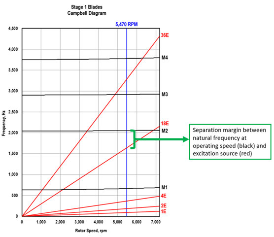
Considering an axial compressor blade as an example, the task usually becomes one of altering the structure of the blade to alter its stiffness and mass. The combined effect results in natural frequencies shifting to higher or lower values. The goal is to shift these frequencies such that they remain sufficiently far away from any identified excitation sources. However, this simple game of avoidance becomes more complicated when one has to consider the actual response shapes of the blade’s natural frequencies in comparison to the nature and shapes of the excitation sources. Moreover, the ability to simply move these natural frequencies around by altering the design becomes further complicated by design constraints such as aerodynamic performance, weight, clearance, geometry, structural integrity, etc.
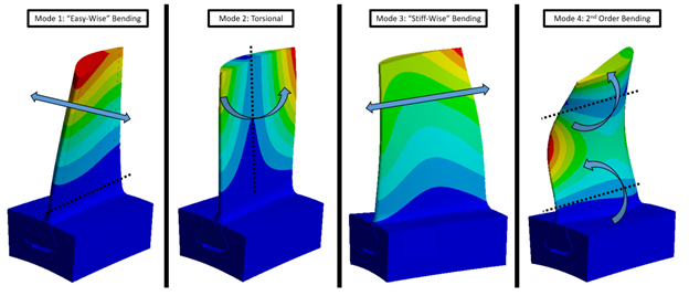
Not all natural frequencies are created equal and each natural frequency identified has its corresponding response shape or mode shape. For example, the first four mode shapes for a typical axial compressor blade are shown below.
It’s quite commonplace throughout the industry to calculate these mode shapes using finite element analysis software. The finite element method lends itself quite well to predicting both the frequencies and corresponding mode shapes for a given structure (as long as the user can provide the correct inputs). However, situations arise when the correct inputs are difficult to provide for a finite element model. In certain situations, it becomes necessary to correlate not only the predicted natural frequencies from a finite element model to the experimentally measured frequencies but also to correlate the predicted mode shapes with experimentally measured mode shapes. The ability to experimentally measure a structure’s mode shape is less commonplace and a more involved task that requires an in-depth testing process, additional tools, and more expertise. For these reasons, RMS has limited the majority of its frequency testing to experimentally measuring natural frequencies and correlating those frequencies to frequencies predicted using finite element modeling. As demand grows for a deeper understanding of vibrations, mode shapes, and how structures actually respond to real-world excitations, RMS has taken steps to meet this demand by expanding its frequency testing capabilities. Using improved technology and testing methods, RMS can now measure frequency response functions and mode shapes through physical testing.
RMS employs several methods and tools to experimentally measure mode shapes. The first step in the process involves performing a “roving accelerometer” or “roving impact” test to measure the frequency response at several locations on a physical part. In the axial compressor blade example, this involves measuring the response to a controlled excitation on a compressor blade at a specific location using an accelerometer. One then “roves” or moves the accelerometer to another location on the blade, repeats the excitation, and measures the response at the new location.
The procedure requires precise application as the tester needs to place the accelerometer at key locations on the structure to properly measure the response. Alternatively, one can employ the principle of “Maxwell’s reciprocity”, and rove the excitation (impact hammer) location while leaving the accelerometer stationary. However, extreme caution must be taken when using Maxwell’s reciprocity with rotating machinery as the assumptions behind it are violated once the machine is set in motion.
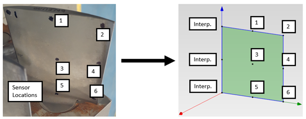
In most cases, sensor locations can be determined using a Modal Assurance Criteria tool. However, for the current compressor blade demonstration, a simple grid of sensor locations was adequate for resolving the easy-wise bending modes. The real blade with associated sensor locations marked is shown below on the left. A “skeleton” or flat wire-frame model of the blade is shown with the same measurement locations on the right.
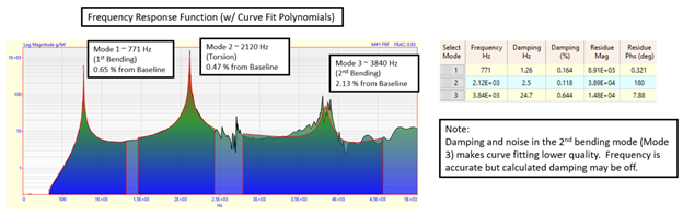
Accessibility can be a challenge with sensor and impact sites. Interpolation is often used between measurement locations and locations where the tester could not gain access. From each measurement location, valuable frequency information is obtained in the form of a Frequency Response Function or FRF. The Frequency Response Function has certain characteristics that allow the calculation of the structure’s natural frequencies, and when combined with the FRFs at other measurement locations on the blade, this information can be used to calculate the actual mode shapes. A side benefit of measuring the FRFs and curve fitting specialized polynomials to these functions is the ability to calculate the structural “damping” associated with each natural frequency. Damping can be difficult to calculate for certain modes and largely depends on how close the polynomial can approximate or “fit” to the measured FRF. Shown below is a typical FRF measured at one location on the blade shown above. Not all FRFs are identical and across different blades, not all modes necessarily occur in the exact same order (The stiff-wise and 2nd order bending modes often switch places depending on the structural characteristics of the blade).
For each location or grid test point on the blade, a frequency response function like the one above is created. Polynomials are fit to the peaks in the frequency response function (the peaks are the resonances or natural frequencies of the structure at that location). With these polynomials, a quantity called a “residue” is calculated. These quantities are then “mapped” onto the skeleton model shown previously. Frequency response functions and curve fits are assigned to each of these measurement points or grid points on the skeleton model. In between these grid points, interpolations are performed and sometimes additional guidance is necessary for the interpolations depending on how many test points were created (in general, the more test points, the better the quality of the interpolation). Finally, with this information, the mode shape can be calculated based on the FRFs and calculated “residues”. Two of the measured mode shapes are shown below for the test blade shown previously:
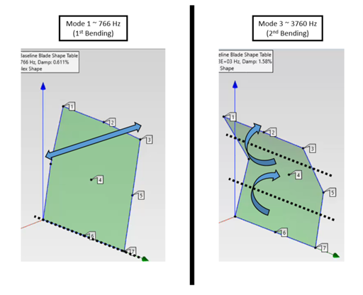
The two modes measured from the test correlate to the fundamental “Easy-Wise Bending” and “2nd Order Bending” modes shown previously. New possibilities arise from being able to experimentally measure mode shapes.
For the first time, RMS can correlate predicted FE frequencies and mode shapes to improve the accuracy and fidelity of FE models. Additionally, damping can be experimentally calculated and used to calibrate and improve FE model accuracy. The experimentally measured mode shapes also provide an opportunity to determine mode shapes for complex assemblies where FE models are not available or possible due to configuration… Furthermore, RMS design engineers can pursue more targeted frequency tuning and optimizations based on experimentally measured mode shape data, and ensure that not only frequencies were altered as desired, but actual mode shapes were altered in a more favorable way. This paves the way for new and exciting innovations when it comes to frequency tuning and design at RMS.